Descriptive Analysis with Python
Python installation
You can install python in different way. For someone who are not familiar with python, feel free to follow these steps:
- Download python @ https://www.python.org/downloads/
- Install it by double click the installer
- Check if the installation success by typing
python3in CMD (Windows) or terminal (Mac or Linux)
1. Download and install VS Code
2. Check python and jupyter package
Make sure you have installed python and jupyter package (see previous slide)
@ Terminal or CMD or Python
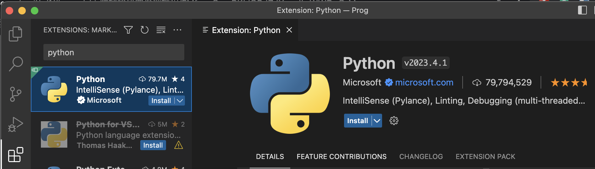
3. Install Python extension
In VS Code, click Extensions, search python, and install the extension
 Jupyter extension is also useful
4. Trust your workspace
Click trust and add the folder with codes in the trust workspace
5. Create a Jupyter Notebook
- by running the Create: New Jupyter Notebook command from the Command Palette (⇧⌘P)
- by creating a new .ipynb file in your workspace

6. Now we are ready to start!

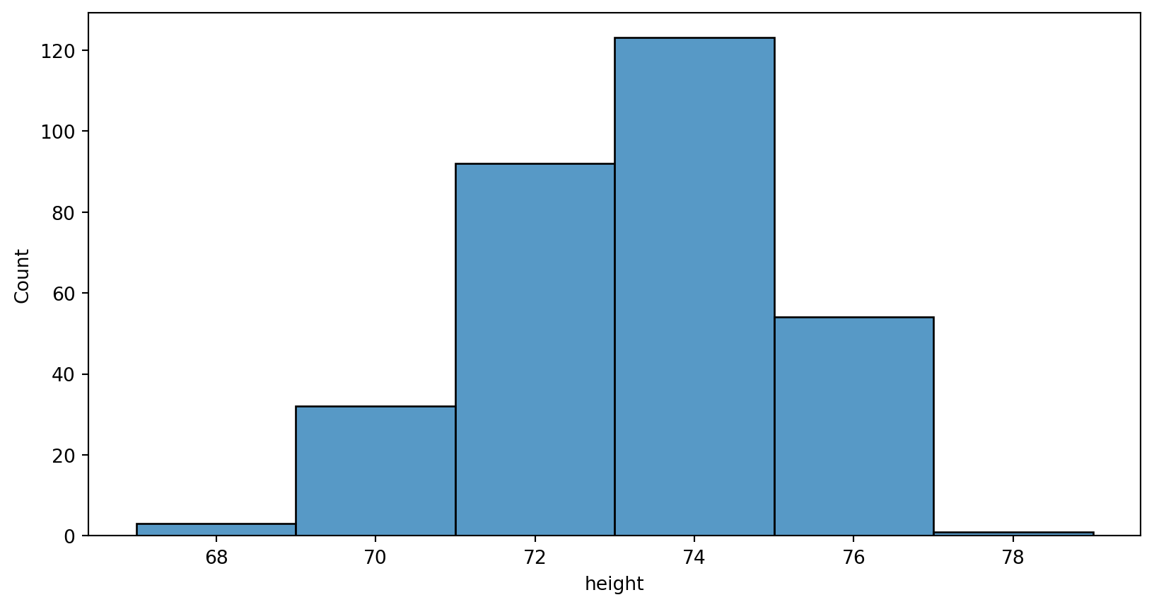
Histogram
histplot(data=your data frame,x=x axis)from seaborn
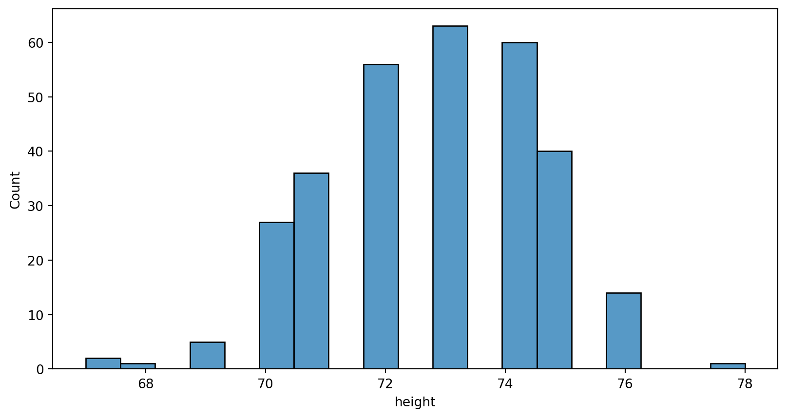
Histogram - bin width
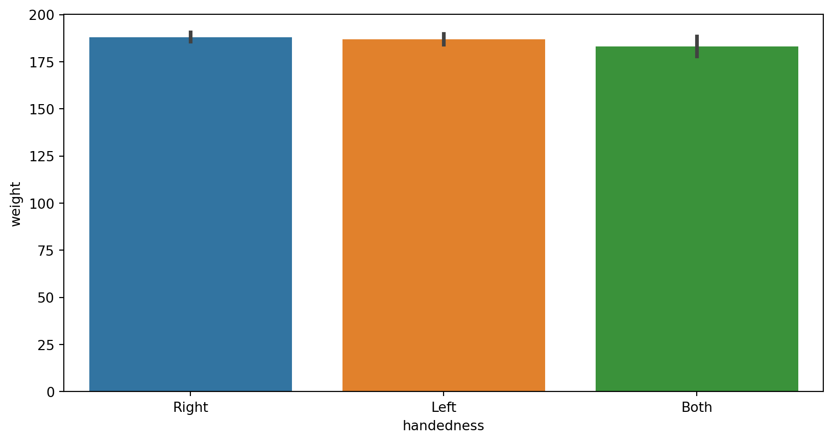
Bar chart
barplot(data=your data, x=x axis, y=y axis)from seaborn
Box plot
boxplot(data=your data, x=x axis, y=y axis)from seaborn
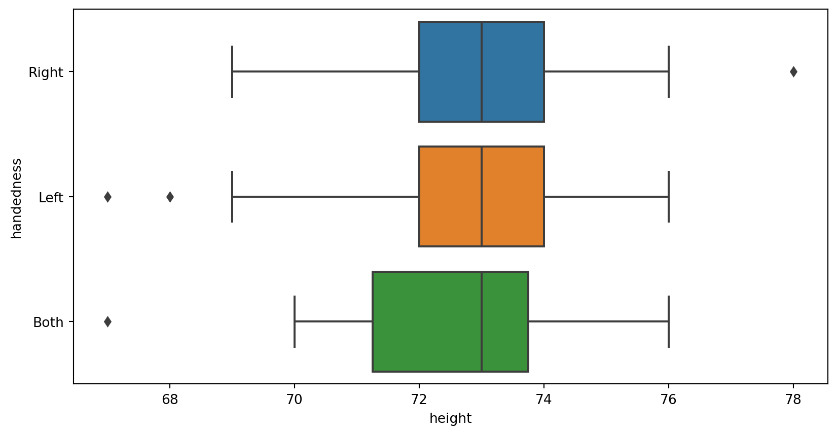
Example
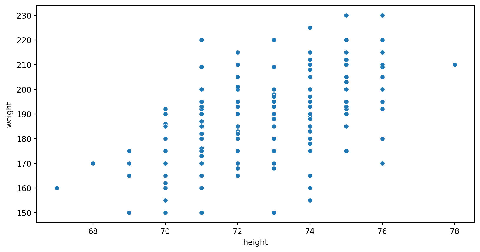
Scatter plot
scatterplot(data=your data, x=x axis, y=y axis)from seaborn