Random Variable and Distribution
Probability (area under the pdf)
statistic (as st) package’s function:
NormalDist(mu=μ, sigma=σ).cdf(x)
Probability (area under the pdf)
Quiz 3-3
You work in Quality Control for GE.
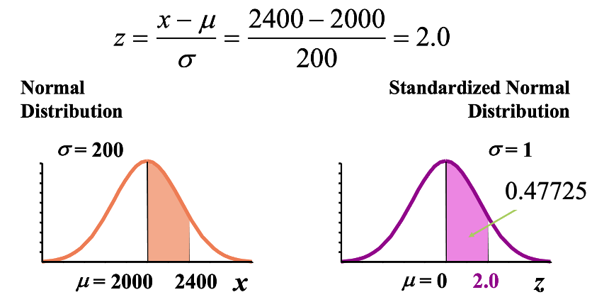
Light bulb life has a normal distribution with μ = 2000 hours and σ = 200 hours.
What’s the probability that a bulb will last
A. between 2000 and 2400 hours?
Quiz 3-3
You work in Quality Control for GE.
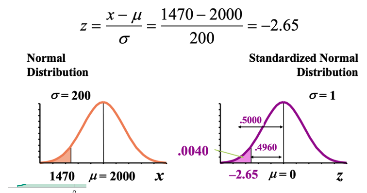
Light bulb life has a normal distribution with μ = 2000 hours and σ = 200 hours.
What’s the probability that a bulb will last
B. less than 1470 hours?
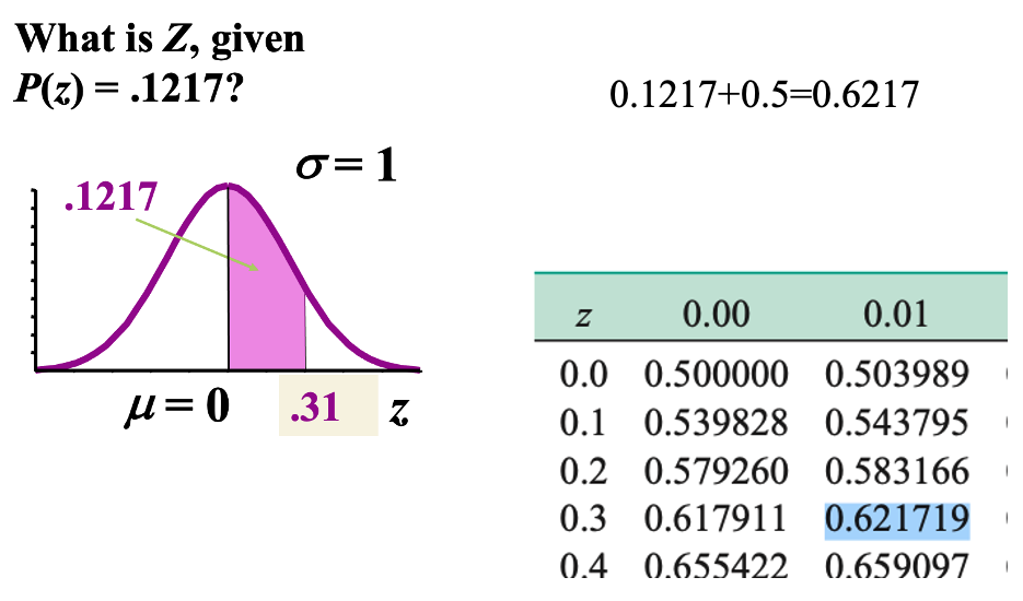
Finding z-Values for Known Probabilities
statistic (as st) package’s function
NormalDist(mu=μ, sigma=σ).inv_cdf(p-value)
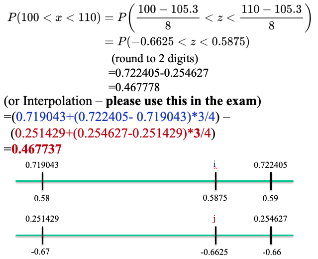
Quiz 3-4
For a particular generation of the tomato plant, the amount x of miraculin produced had a mean of 105.3 and a standard deviation of 8.0. Assume that x is normally distributed.
- Find P(100 < x < 110)
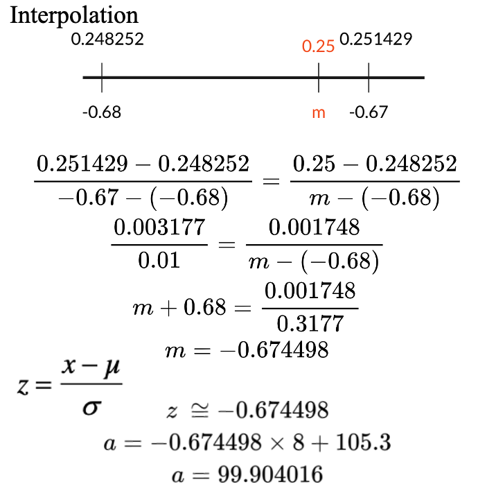
Quiz 3-4
For a particular generation of the tomato plant, the amount x of miraculin produced had a mean of 105.3 and a standard deviation of 8.0. Assume that x is normally distributed.
- Find the value a for which P(x < a) = 0.25
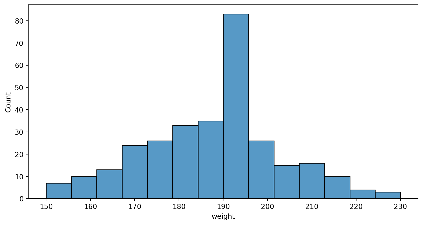
Normal Probability Plots - Histogram
seaborn package’s
histplot(data=your data frame,x=x axis)
Normal Probability Plots - PP
With scipy package’s stats, we can use function probplot(data, plot=sns.mpl.pyplot) to draw Probability Plots
<Figure size 960x480 with 0 Axes>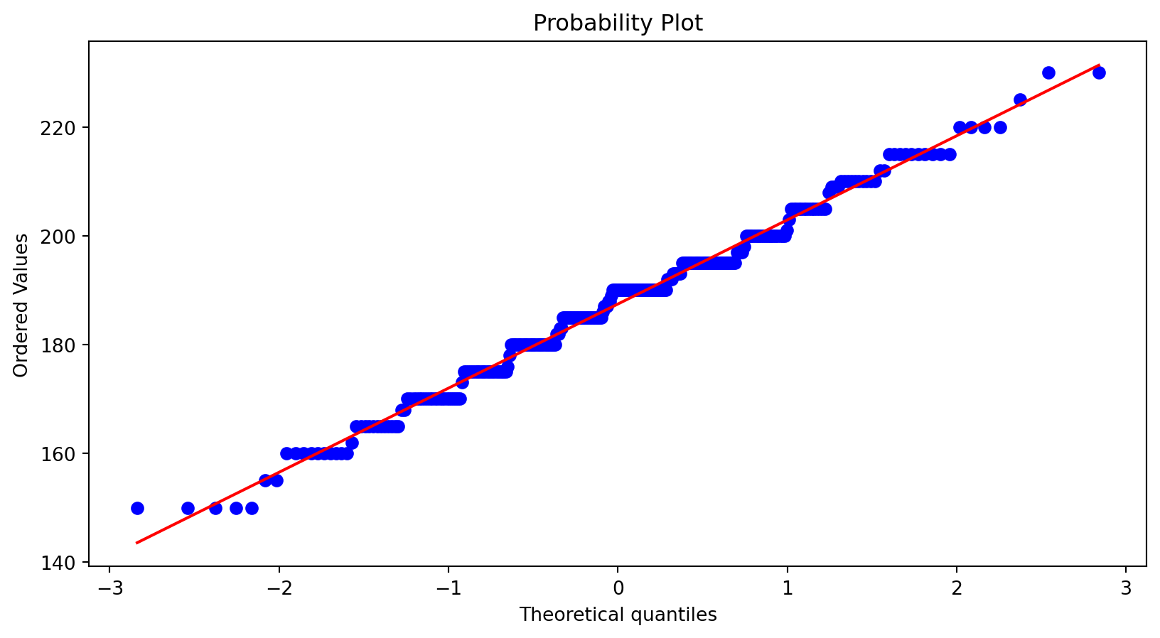
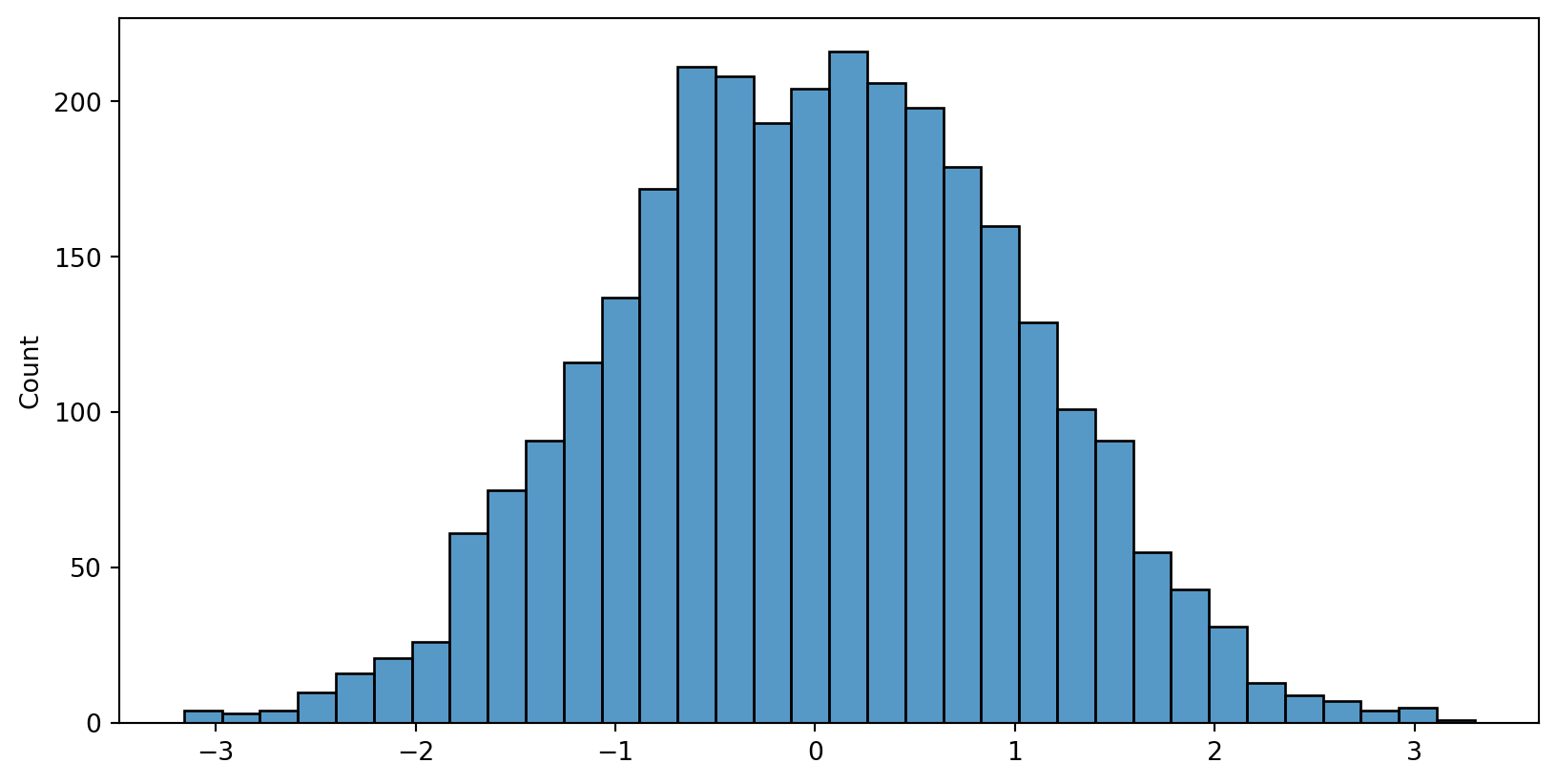
Normal Probability Plots - Histogram
numpy’s function random.normal can be used to generate data with normal distribution
Normal Probability Plots - PP
With scipy package’s stats, we can use function probplot(data, plot=sns.mpl.pyplot) to draw Probability Plots
<Figure size 960x480 with 0 Axes>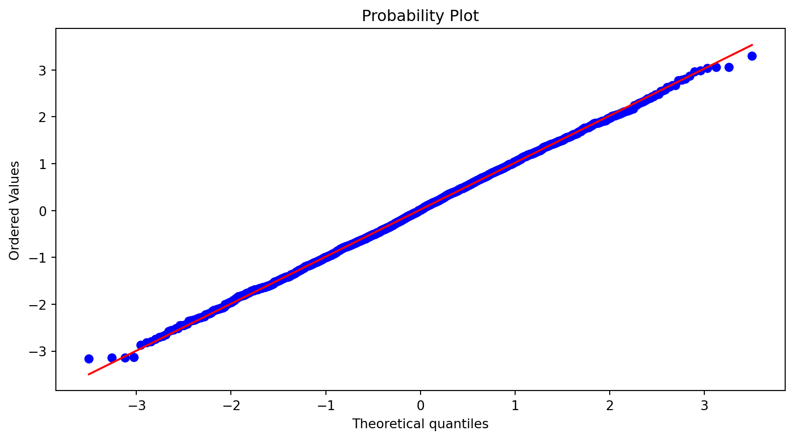
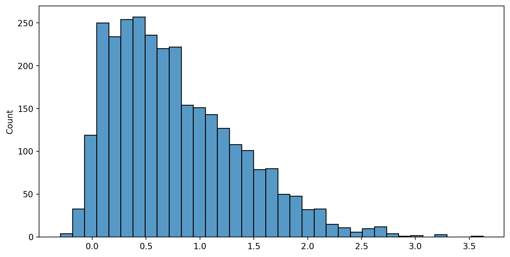
Normal Probability Plots - Histogram
With scipy package’s stats, we can use function skewnorm.rvs() to generate skewed data
Normal Probability Plots - PP
<Figure size 960x480 with 0 Axes>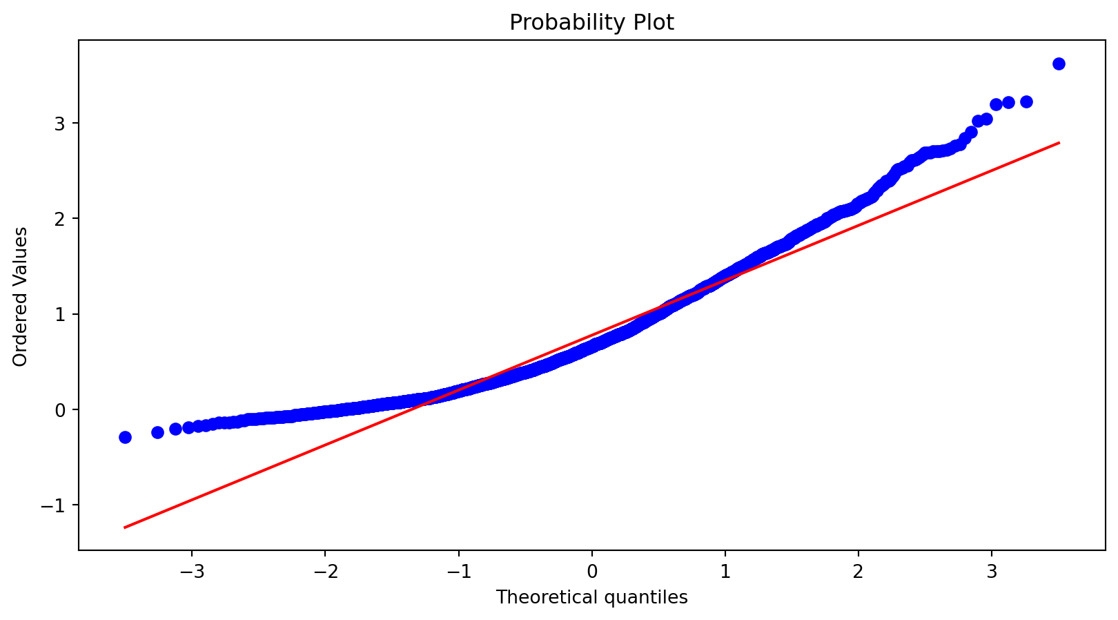
Binomial Distribution - pmf
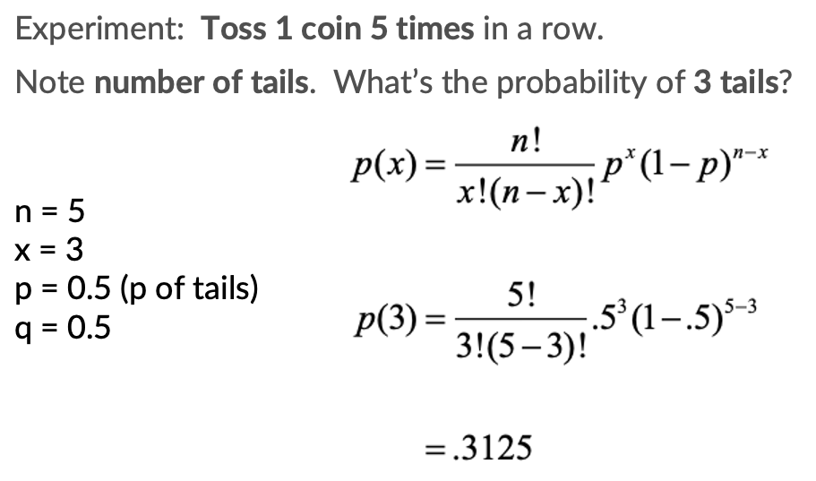
- n: number of trials
- x: number of success
- p: Probability of a ‘Success’ on a single trial
Binomial Distribution - pmf
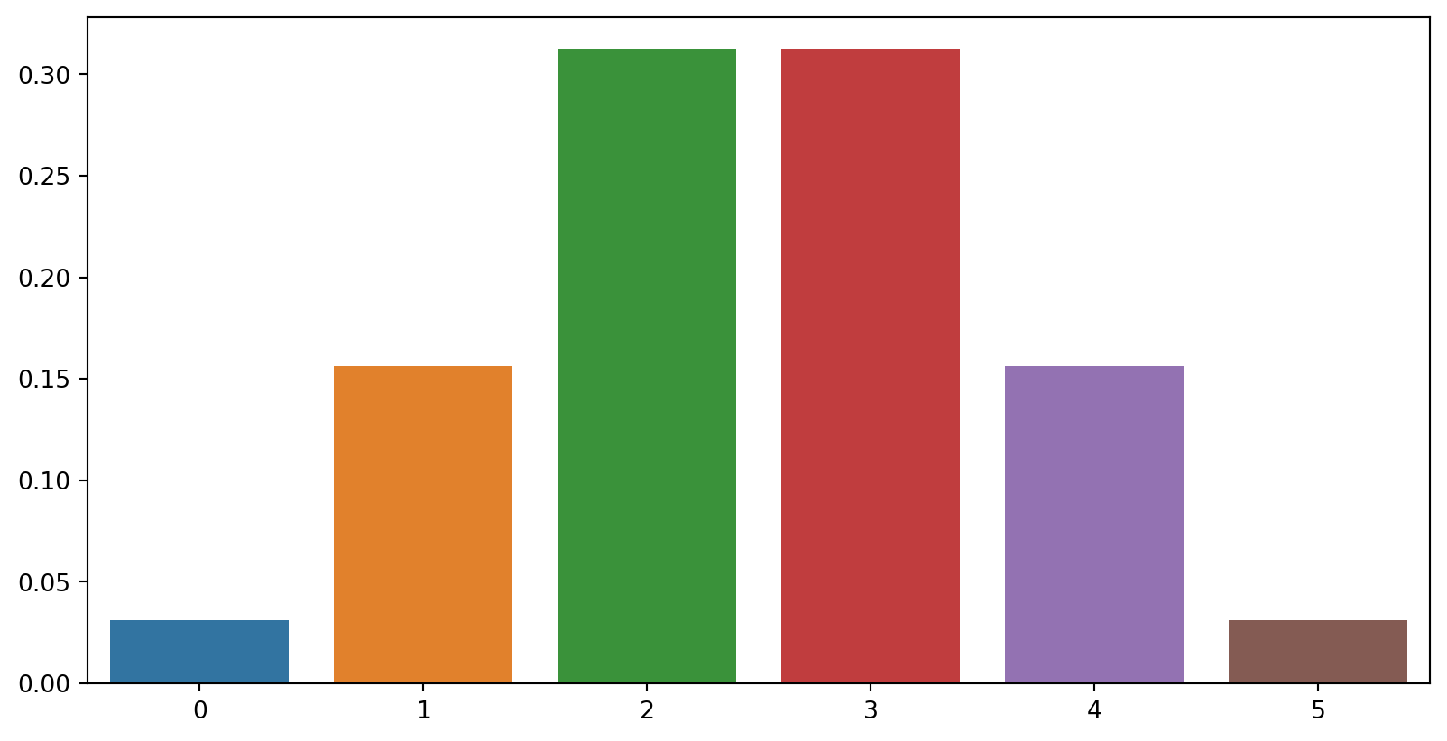
Probability (sum of the pmf)
With scipy package’s stats:
binom.pmf(x, n, p)
Probability (sum of the pmf)
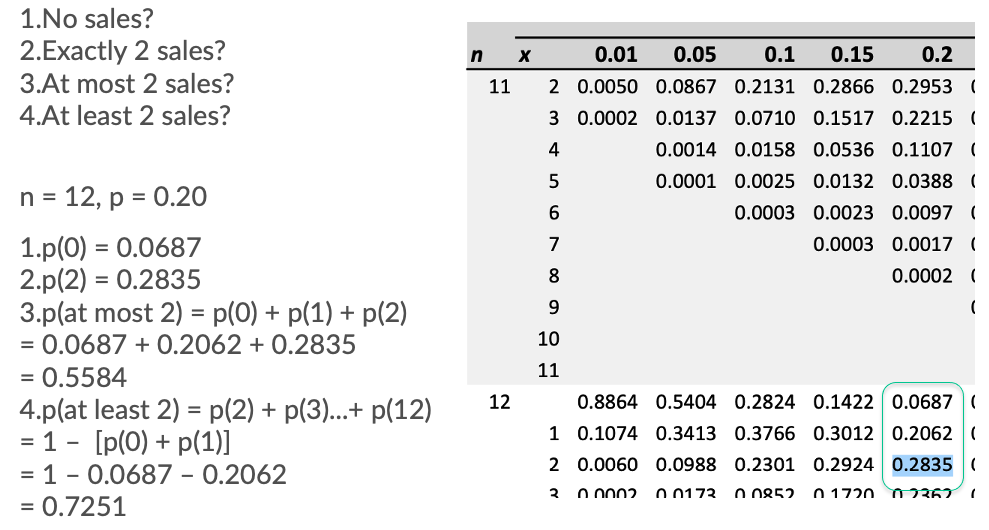
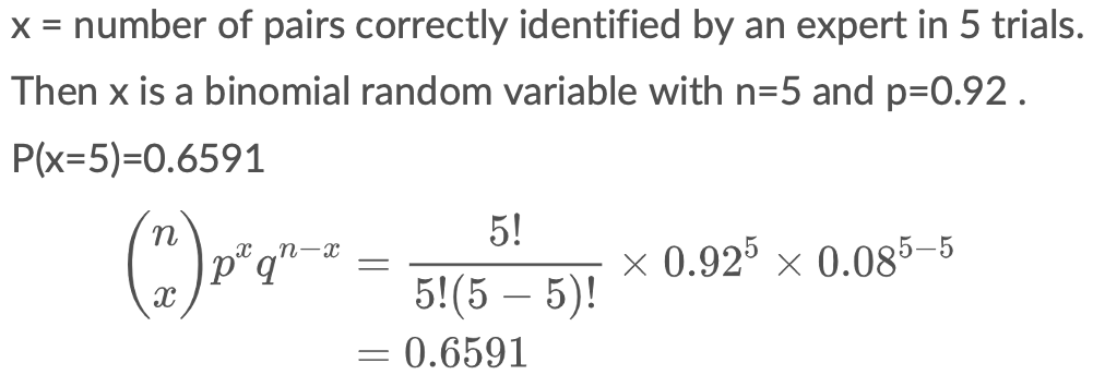
0.5583457484800001Quiz 3-6-a
The study found that when presented with prints from the same individual, a fingerprint expert will correctly identify the match 92% of the time.
- What is the probability that an expert will correctly identify the match in all five pairs of fingerprints?
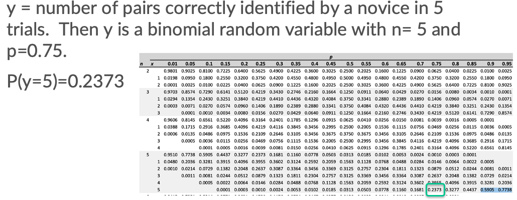
Quiz 3-6-b
In contrast, a novice will correctly identify the match 75% of the time. Consider a sample of five different pairs of fingerprints, where each pair is a match.
- What is the probability that a novice will correctly identify the match in all five pairs of fingerprints?
Poisson Distribution - pmf
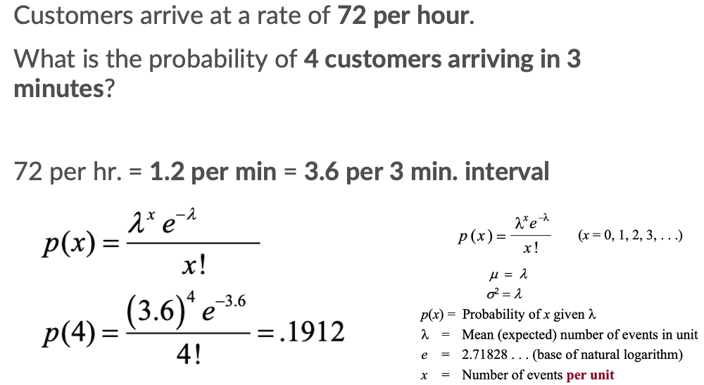
Poisson Distribution - pmf
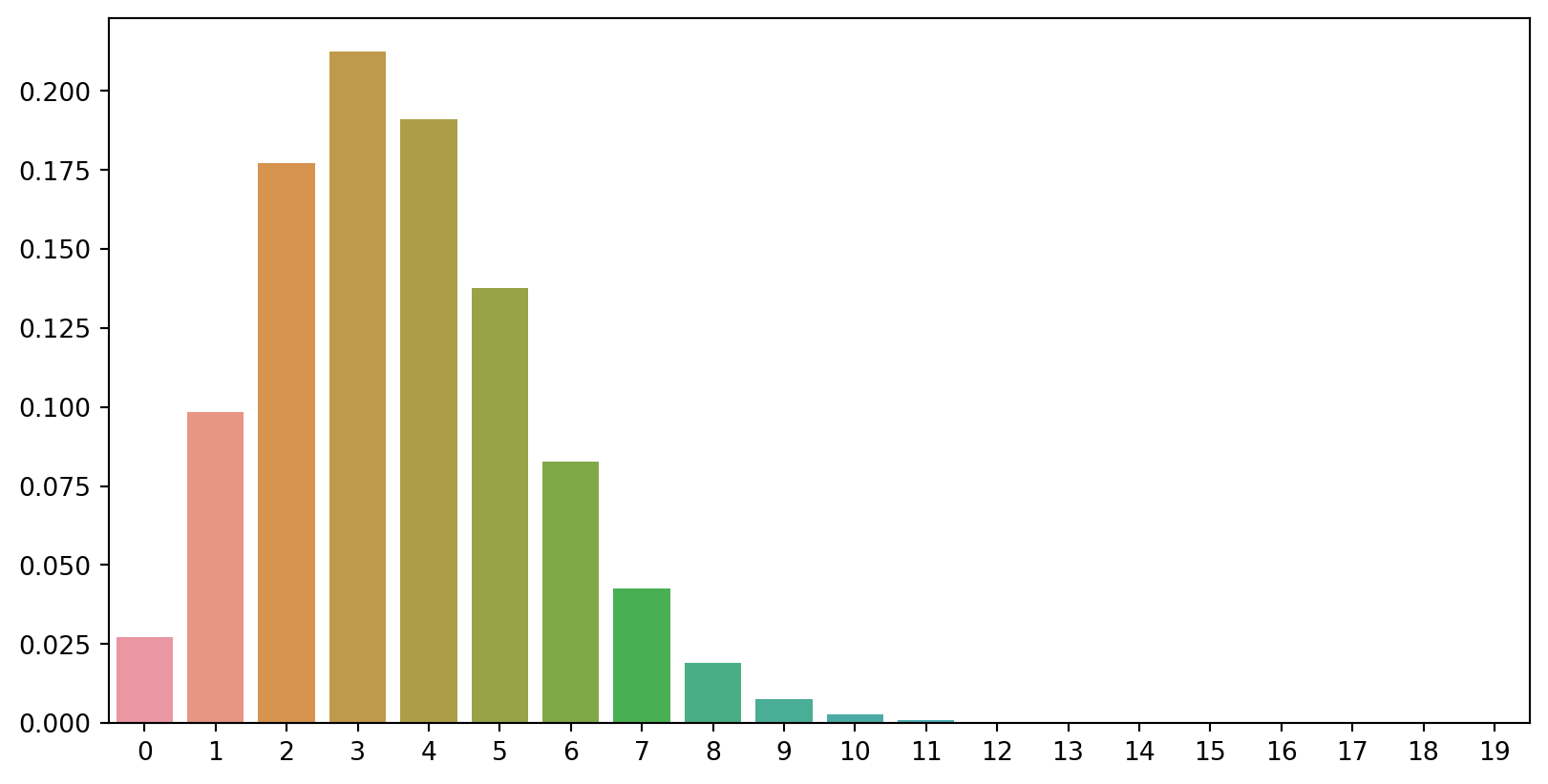
Probability (sum of the pmf)
With scipy package’s stats:
poisson.pmf(k=x, mu=λ)
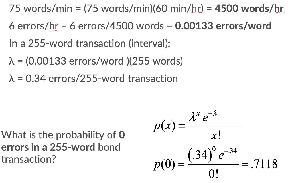
Quiz 3-8
You work in Quality Assurance for an investment firm. A clerk enters 75 words per minute with 6 errors per hour.
Probability (area under the pdf)
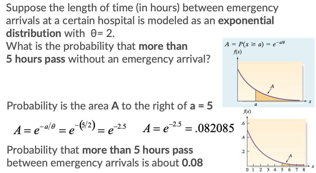
With scipy package’s stats:
expon.cdf(x, scale=θ)
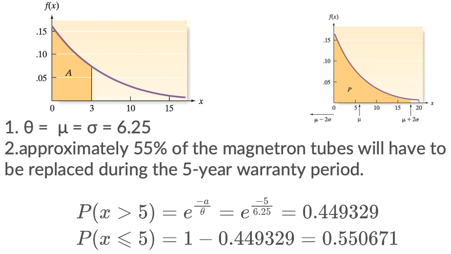
Quiz 3-9
the length of life of a magnetron tube has an exponential probability distribution with θ = 6.25.
Suppose a warranty period of 5 years is attached to the magnetron tube. What fraction of tubes must the manufacturer plan to replace?